Porkchop plots

Other application for Lambert problem solvers is plotting so-called porkchop plots or delta-v maps.

Porkchop plot is a chart shows level curves of characteristic energy required for a transfer to a target within a range of given dates of departure and arrivals.

Characteristic energy can be expressed as:

This is complex characteristic, representing the shape of the orbit, total energy (implies delta-v) required for build it, etc.

Typical porkchop plot looks like this:

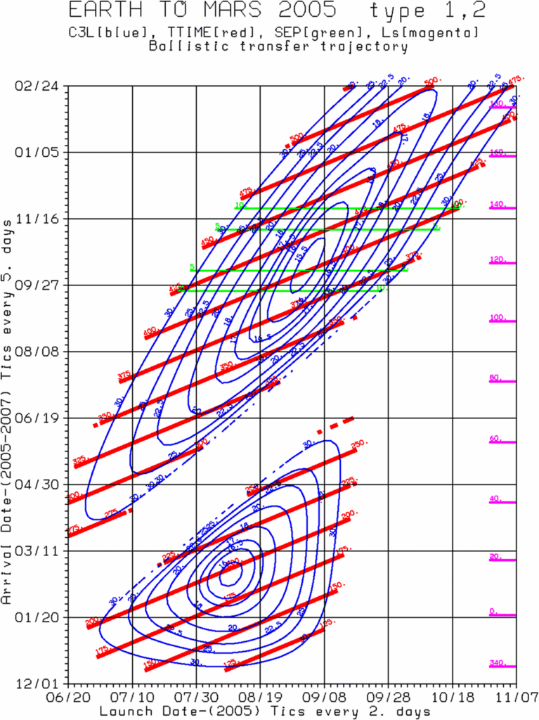
As you can see, it’s pretty complex graph, representing not only $C_3$ changes and “sweet spots”, but also time of flight, and lot of other information. Note, that porkchop plot uses absolute time scale (real dates).

Such complex and aesthetic representation may be required for top experts and important pitches, but in everyday work it’s more convenient to use simpler forms.

One of these forms are delta-v maps.

Delta-v maps

By sense, it’s almost the same thing as porkchop plot. But on delta-v map we typically representing not $C_3$ but sum of $\Delta v$ required for transfer, and typically using relative, not absolute, time.

For example, recall our previous problem from my article about Lambert problem solutions. There we have $h_{int} = 300$ km,$h_{tgt} = 3000$ km, and phase angle $\vartheta = 90^\circ$ (interceptor is forward from target). So, for this problem delta-v map will look like this:

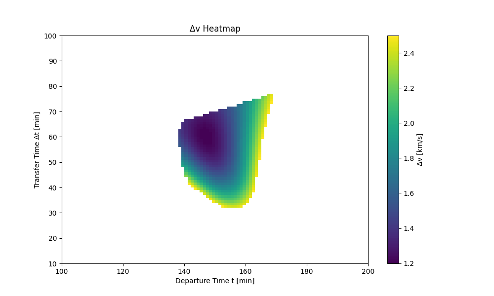
This map is built by my self-made astrodynamics tools software library, based on methods and algorithms from “Fundamentals of Astrodynamics and Applications”, Fourth Edition, by David Vallado and other textbooks (incl. “An Introduction to the Mathematics and Methods of Astrodynamics, Revised Edition” by Richard H. Battin, “Satellite Orbits. Models, Methods and Applications” by Oliver Montenbruck & Eberhard Gill, and other).

Here on horizontal axis we have relative departure time (calculated from the moment of known spacecraft state), and on vertical axis we have transfer time (duration of flight between insertion and exit maneuvers of a transfer).

Color spots represents total $\Delta v$ required for the operation. Darker the color less $\Delta v$. White color represent $\Delta v$ higher the boundary level (in this case 2.5 km/s).

Usage of delta-v maps for maneuver optimization

One of the most important applications of delta-v maps is to use them for search for launch windows (or, speaking wider – for optimal transfers).

As an example, let’s look on the problem described above. On Fig. 2 it’s visible (with “naked eye”) that closest opportunity for insertion into intercept maneuver will be at about 140-160 minutes from known (given) state, and a transfer will require something about 40-70 minutes.

Let’s change calculation parameters and set departure time and transfer time constraints as mentioned above, with step 60 seconds. We will get next picture (Fig. 3):

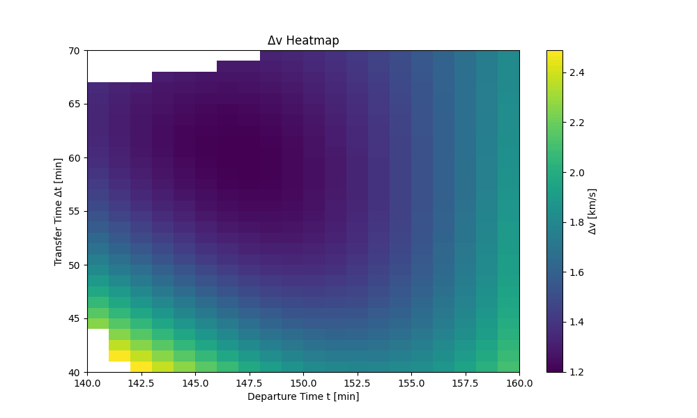
Here it’s visible that “sweet spot” for departure is somewhere between 146 – 148 minutes and best transfer time should be about 59 – 61 minutes.

Let’s change calculation constraints again to match received parameters, and for this time set check step 12 seconds (0.2 minute). Additionally, let’s reduce $\Delta v$ boundary from 2.5 km/s to 1.25 km/s. This changes will help us get higher resolution. We will get next picture (Fig. 4):

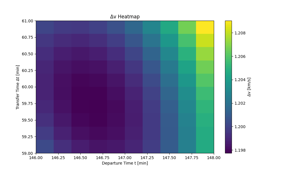
Now, applying threshold filtering to this picture (even in image editor like GIMP or Photoshop – I like this simple graphical magic!), we will easily get this (Fig. 5):

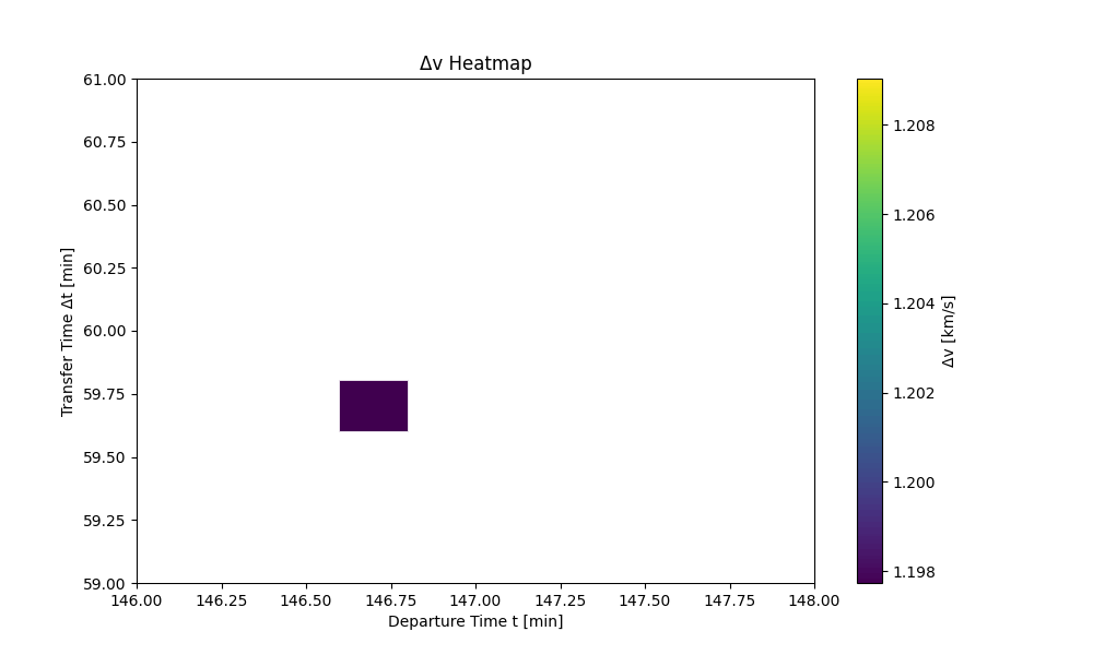
So, here we can see (again, with “naked eye”) that optimal departure time is ~146.7 minutes from given state, and optimal transfer time is ~59.7 minutes.

Let’s enter this parameters in this with propagator. And we have this (Fig. 6):

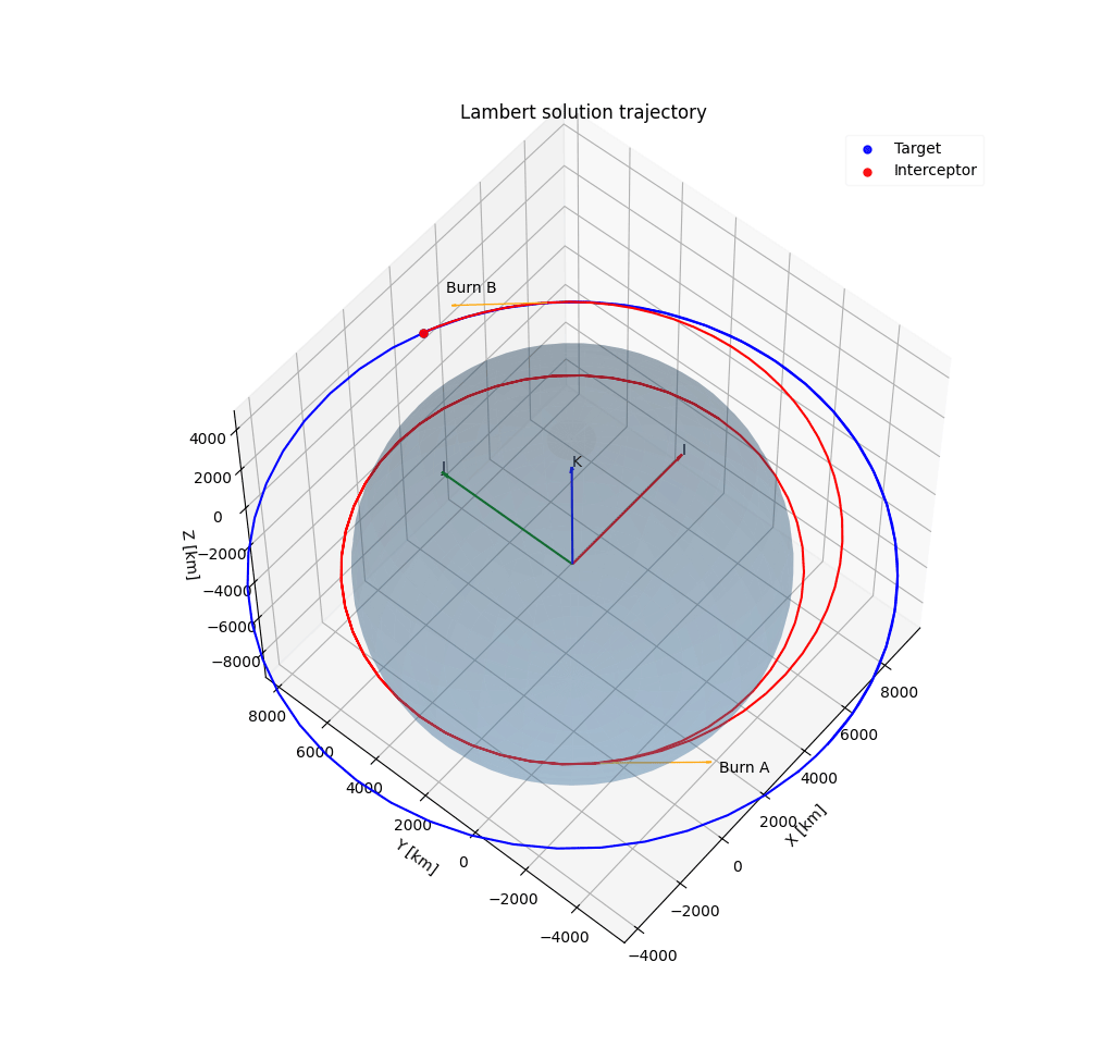
On Fig. 6 we can see almost perfect Hohmann transfer. Vectors of burns A and B are almost perfectly tangential to orbit curve, total $\Delta v = 1.198$ km/s.

Hohmann transfer calculation algorithm returns absolutely same values:

deltav [km/s]: 1.198
tautrans [min]: 59.7

Main advantage

Someone may ask – why to use this all if we have simple Hohmann formulas? The answer is that with Hohmann transfer you can calculate only theoretically optimal transfer between circular orbits.

With Lambert problem solver and delta-v map you can calculate real (almost) optimal transfer between any orbits.

Final note

Saying “almost” I meaning that Lambert problem solution is not absolutely precise. This is still an approximation, working in two-body dynamics without getting in count gravity pulls of other bodies and other effects like atmospheric drag or solar wind pressure.

So in practice without additional corrections it works good only for relatively short transfer arcs away from strong perturbation sources. In other cases it should be used as a first step, providing good initial data for further numeric integration.