Preface

When people talk about space navigation and orbital maneuvers, they often refer to classic solutions like the Hohmann transfer. While these are foundational tools in the astrodynamicist’s toolkit, in practice astrogators prefers more advanced solutions.

One of them, used especially for high-level mission planning, is a solving of Lambert problem.

The Subject

Originally, Lambert problem was posted by Swiss mathematician Johann Heinrich Lambert at 1761. Originally, problem was about determination of parameters of the orbit between two known points, getting in count a time of flight between this points. It’s solution was needed for studying orbits of celestial bodies (by sense, for initial orbit determination from measurements gathered from observations).

In astrodynamics, solutions of Lambert problem also widely used in solutions of targeting problem, i.e., for plotting of intercept and rendezvous maneuvers.

Principle

By sense, Lambert problem is the boundary valve problem for the differential equation

or, if to express it with words, solution of Lambert problem determines amount of acceleration required for transfer between two positions of celestial body in given time.

For targeting problem, we solving Lambert problem to find combination of two velocity changes ($\delta \vec{v_0}$ and $\delta \vec{v_1}$) allowing to perform transfer between spacecraft states $\begin{bmatrix} \vec{r_0} & \vec{v_0} \end{bmatrix}$ and $\begin{bmatrix} \vec{r_1} & \vec{v_1} \end{bmatrix}$ in given time $t$.

Practical application

In practice Lambert problem typically solving numerically. These freeform, non-tangential, fully three-dimensional maneuvers allow for precise, efficient, and sometimes dramatic intercepts. It’s not just transfer – it’s targeting with deadly precision of an eagle striking from the sunlight.

On the images below you can see an example of a two impulse chain of intercept/rendezvous maneuvers, developed by solving Lambert (targeting)problem.

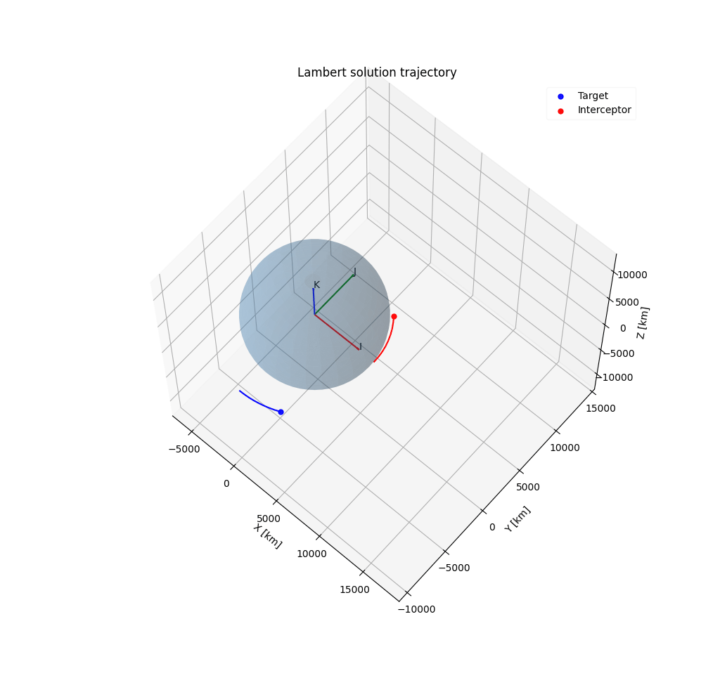
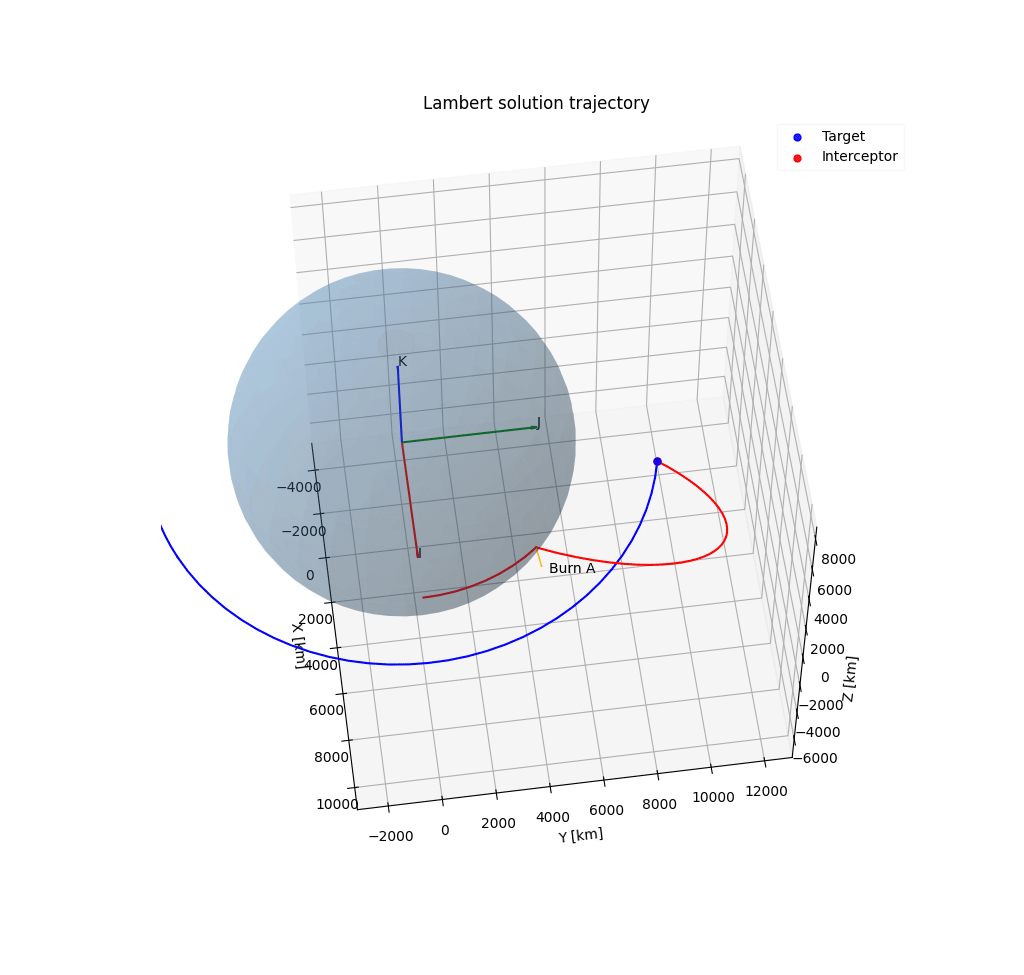
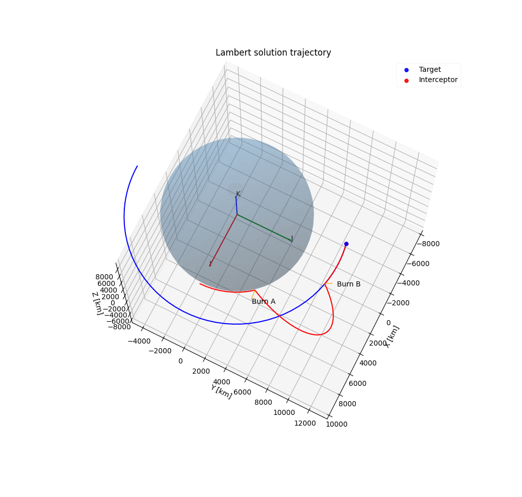
Note the dramatic curve of red (interceptor) trajectory!

Of course, this is very exaggerated example – this rendezvous required total $\Delta v = 14.504$ km/s. This was made on purpose, to demonstrate the principle of the process. In practice, of course, everything is much more prosaic.

For example, like on next picture.

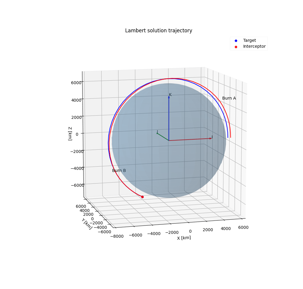
Here you can see target and interceptor on near-polar orbit. The intercept started from SSO with $h=894$ km to SSO with $h=567$ km. Required $\Delta v$ was 644 m/s. Note, that between burns A and B interceptor trajectory (red) goes below target trajectory! This can be dangerous, especially in LEO. Multiple times check boundaries of your problem, propagators and force models you using, because in other cases you very possibly will face troubles!

And finally, note one other specific kickback of targeting by solving Lambert problem. The solution of Lambert problem does not suggest optimal transfer – it provides the one and only possible within given constraints. So, in some cases, it can provide solutions like those presented on next pictures.

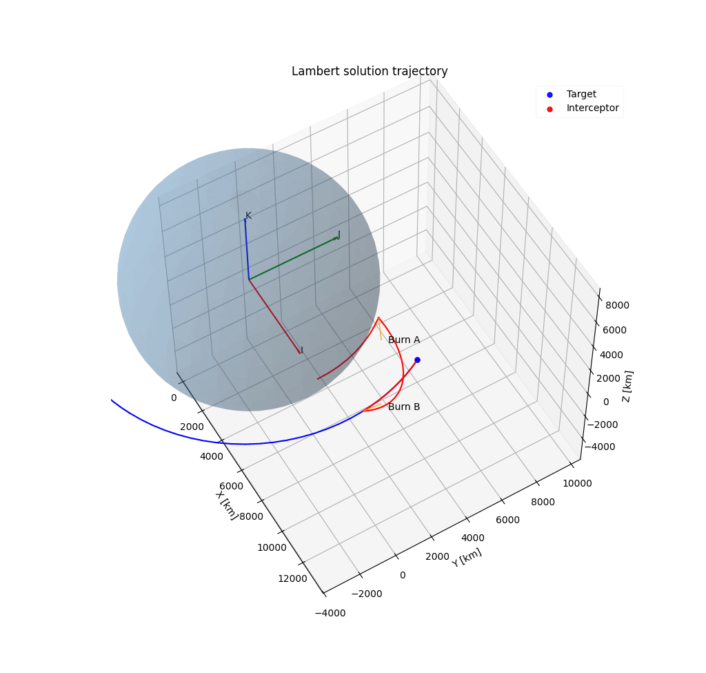
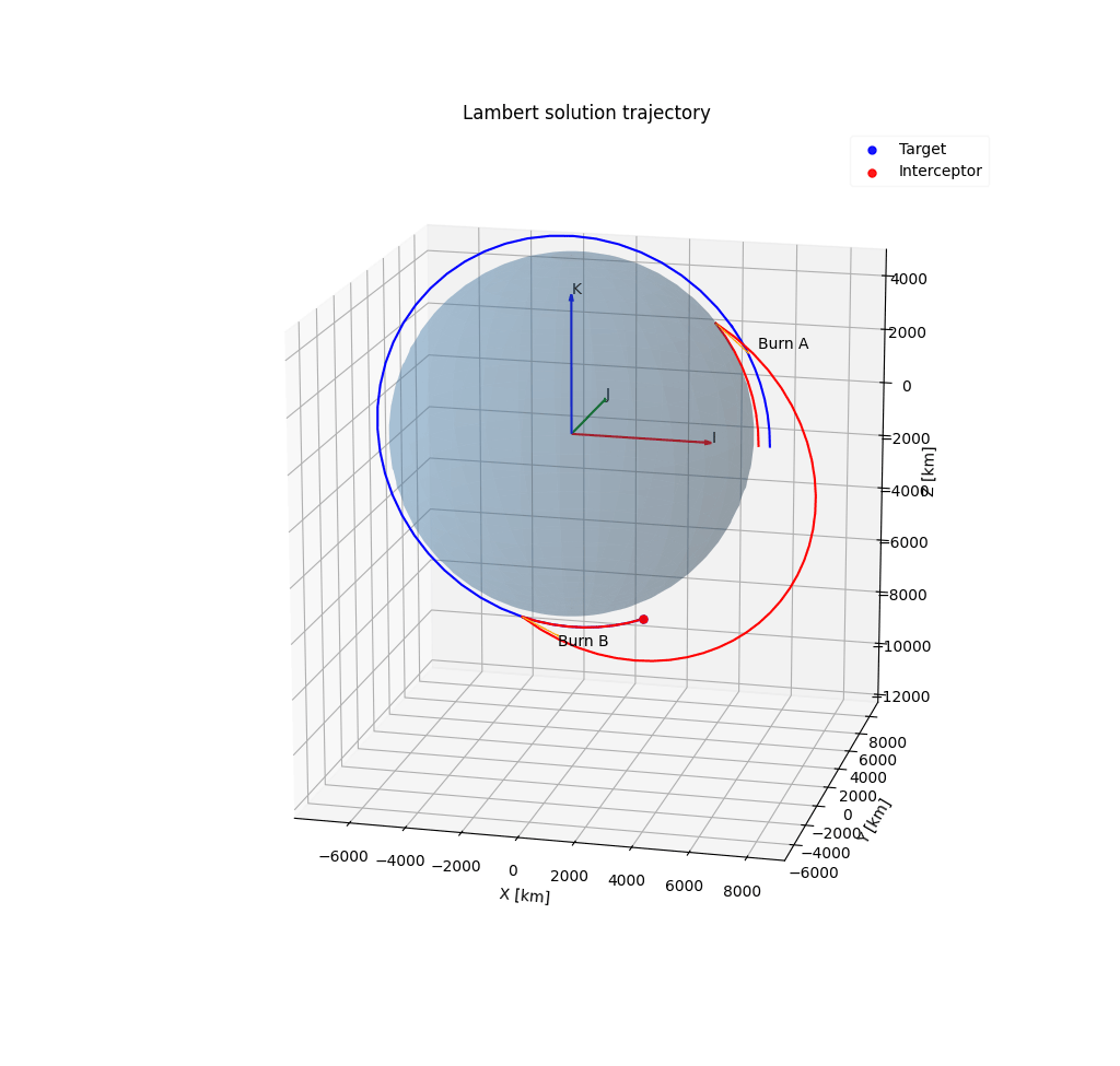
Looks very cool! But, of course, in reality it is not possible even with a torchship like Project Orion or Zubrin’s nuclear salt-water rocket.

Software & Algorithms

To plot this transfers, I used my own C++/Python software library for solving astrodynamic problems.

Algorithms for solving Lambert problem are based on algorithms from the book “Fundamentals of Astrodynamics and Applications”, Fourth Edition, by David Vallado.

In addition to this, I am planning to implement in my library Izzo algorithm developed by Dario Izzo.