
Preface
As I mentioned in the post about my astrodynamics tools library, I undertook a research to validate correctness of my software.
Because I am following the educational trajectory from “Fundamentals of Astrodynamics and Applications”, Fourth Edition, by David A. Vallado, my astrodynamics algorithms library based mostly on algorithms from this textbook.
But my practice showed, that even famous textbooks can contain errors, and even without them, practical application of described methods may have specific traits.
So because of this I decided to cross-test algorithms from my astrodynamics library on exercises from other known textbook “Satellite Orbits. Models, Methods and Applications” © 2000 by Oliver Montenbruck & Eberhard Gill.
Exercises
Below, I provide listings of solutions of an exercises from the textbook, with my comments.
Exercise 2.1 – Hohmann transfer calculation
Using HohmannTransfer algorithm from “Fundamentals” – very simple
Running Exercise_2_1.py...
-----------------------------------
Source of examples:
Oliver Montenbruck • Eberhard Gill
Satellite Orbits
Models, Methods and Applications
-----------------------------------
Results:
+------------------+--------------+--------------+
| Parameter        |   Ref. value |   Calculated |
+==================+==============+==============+
| dv total, (km/s) |      0.01308 |      0.01308 |
+------------------+--------------+--------------+
Execution time: 0.000054 s.Exercise 2.2 – Kepler equation solver performance
I am using Kepler equation solver provided in “Fundamentals”. So I can not complete the test exactly like required in the textbook. But still:
Running Exercise_2_2.py...
KepEqtnE iteration limit reached
KepEqtnE iteration limit reached
KepEqtnE iteration limit reached
KepEqtnE iteration limit reached
Results:
+-----------+-----------+---------------+---------------+------------+------------------+
|   M (deg) |   Iter. # |    Eref (rad) |       E (rad) |   ΔE (rad) |   Exec. time (s) |
+===========+===========+===============+===============+============+==================+
|       4.0 |         1 | 0.24318719633 | 0.24854417699 |  5.357e-03 |         0.000388 |
+-----------+-----------+---------------+---------------+------------+------------------+
|       4.0 |         2 | 0.24318719633 | 0.24319554879 |  8.352e-06 |         0.000081 |
+-----------+-----------+---------------+---------------+------------+------------------+
|       4.0 |         3 | 0.24318719633 | 0.24318719639 |  6.000e-11 |         0.000076 |
+-----------+-----------+---------------+---------------+------------+------------------+
|      50.0 |         1 | 1.59249513093 | 1.59249513093 |  0.000e+00 |         0.000074 |
+-----------+-----------+---------------+---------------+------------+------------------+Exercise 2.3 – Calculate osculating elements
Using RV2COE and KepEqtnE from “Fundamentals” easily achievng:
Running Exercise_2_3.py...
Results:
+--------------+---------------+---------------+--------------+
| Parameter    |    Ref. value |    Calculated |   Difference |
+==============+===============+===============+==============+
| a/SMA (km)   | 25015.18      | 25015.18      |    1.846e-05 |
+--------------+---------------+---------------+--------------+
| e/ECC        |     0.7079772 |     0.7079772 |    2.913e-08 |
+--------------+---------------+---------------+--------------+
| i/INC (deg)  |     6.971     |     6.970729  |    2.708e-04 |
+--------------+---------------+---------------+--------------+
| Ω/RAAN (deg) |   173.29      |   173.2902    |    1.632e-04 |
+--------------+---------------+---------------+--------------+
| ω/AOP (deg)  |    91.553     |    91.55289   |    1.127e-04 |
+--------------+---------------+---------------+--------------+
| M/MA (deg)   |   144.225     |   144.225     |    8.808e-06 |
+--------------+---------------+---------------+--------------+
Execution time: 0.000078 s.Exercise 2.4 – topocentric satellite motion
Using modified RAZEL algorithm:
Running Exercise_2_4.py...
Results:

β, el, ρ (azimuth, elevation, slant range) values
+-----------+--------------+-----------+-------------+---------------+------------+--------------+-------------+----------+------------+
|   t (min) |   βref (deg) |   β (deg) |   Δβ, (deg) |   elref (deg) |   el (deg) |   Δel, (deg) |   ρref (km) |   ρ (km) |   Δρ, (km) |
+===========+==============+===========+=============+===============+============+==============+=============+==========+============+
|         6 |        151.1 |     151.1 |   3.734e-02 |          -0.1 |        0.0 |    1.402e-01 |      3644.9 |   3644.9 |  3.582e-02 |
+-----------+--------------+-----------+-------------+---------------+------------+--------------+-------------+----------+------------+
|         7 |        149.8 |     149.8 |   1.922e-02 |           3.5 |        3.7 |    1.882e-01 |      3262.7 |   3262.7 |  2.788e-03 |
+-----------+--------------+-----------+-------------+---------------+------------+--------------+-------------+----------+------------+
|         8 |        148.2 |     148.2 |   1.965e-03 |           7.7 |        7.8 |    1.248e-01 |      2884.1 |   2884.1 |  5.645e-03 |
+-----------+--------------+-----------+-------------+---------------+------------+--------------+-------------+----------+------------+
|         9 |        146.0 |     146.0 |   1.310e-02 |          12.5 |       12.6 |    1.497e-01 |      2512.4 |   2512.4 |  2.685e-03 |
+-----------+--------------+-----------+-------------+---------------+------------+--------------+-------------+----------+------------+
|        10 |        142.9 |     142.9 |   3.943e-03 |          18.3 |       18.5 |    1.648e-01 |      2153.0 |   2153.0 |  4.200e-02 |
+-----------+--------------+-----------+-------------+---------------+------------+--------------+-------------+----------+------------+
|        11 |        138.2 |     138.1 |   5.240e-02 |          25.6 |       25.7 |    1.085e-01 |      1814.8 |   1814.8 |  2.777e-02 |
+-----------+--------------+-----------+-------------+---------------+------------+--------------+-------------+----------+------------+
|        12 |        130.3 |     130.2 |   7.627e-02 |          34.8 |       34.9 |    8.357e-02 |      1514.1 |   1514.0 |  5.734e-02 |
+-----------+--------------+-----------+-------------+---------------+------------+--------------+-------------+----------+------------+
|        13 |        115.6 |     115.4 |   1.801e-01 |          45.8 |       45.8 |    4.893e-02 |      1278.8 |   1278.7 |  5.476e-02 |
+-----------+--------------+-----------+-------------+---------------+------------+--------------+-------------+----------+------------+
|        14 |         86.8 |      86.6 |   2.339e-01 |          54.9 |       54.9 |    2.136e-02 |      1151.0 |   1150.9 |  5.285e-02 |
+-----------+--------------+-----------+-------------+---------------+------------+--------------+-------------+----------+------------+
|        15 |         48.4 |      48.2 |   2.395e-01 |          53.7 |       53.6 |    1.311e-01 |      1167.0 |   1167.0 |  3.677e-02 |
+-----------+--------------+-----------+-------------+---------------+------------+--------------+-------------+----------+------------+
|        16 |         23.0 |      22.9 |   1.059e-01 |          43.6 |       43.4 |    1.646e-01 |      1321.7 |   1321.7 |  2.036e-02 |
+-----------+--------------+-----------+-------------+---------------+------------+--------------+-------------+----------+------------+
|        17 |         10.1 |      10.1 |   6.911e-03 |          32.9 |       32.7 |    1.633e-01 |      1574.2 |   1574.2 |  1.355e-02 |
+-----------+--------------+-----------+-------------+---------------+------------+--------------+-------------+----------+------------+
|        18 |          3.1 |       3.1 |   3.000e-03 |          24.2 |       24.0 |    1.920e-01 |      1884.9 |   1884.9 |  1.776e-03 |
+-----------+--------------+-----------+-------------+---------------+------------+--------------+-------------+----------+------------+
|        19 |        358.8 |     358.8 |   4.073e-02 |          17.3 |       17.1 |    1.861e-01 |      2228.7 |   2228.7 |  2.613e-02 |
+-----------+--------------+-----------+-------------+---------------+------------+--------------+-------------+----------+------------+
|        20 |        356.0 |     356.0 |   3.215e-02 |          11.7 |       11.5 |    1.574e-01 |      2591.4 |   2591.4 |  1.560e-02 |
+-----------+--------------+-----------+-------------+---------------+------------+--------------+-------------+----------+------------+
|        21 |        354.1 |     354.1 |   3.131e-02 |           7.1 |        6.9 |    2.138e-01 |      2965.0 |   2965.0 |  1.594e-02 |
+-----------+--------------+-----------+-------------+---------------+------------+--------------+-------------+----------+------------+
|        22 |        352.6 |     352.6 |   3.852e-02 |           3.1 |        2.9 |    2.320e-01 |      3344.7 |   3344.7 |  3.842e-02 |
+-----------+--------------+-----------+-------------+---------------+------------+--------------+-------------+----------+------------+
|        23 |        351.6 |     351.6 |   3.413e-02 |          -0.5 |       -0.7 |    1.949e-01 |      3727.3 |   3727.4 |  5.388e-02 |
+-----------+--------------+-----------+-------------+---------------+------------+--------------+-------------+----------+------------+

Root Mean Square Error
+----------------+------------------+---------------+
|   RMSE β (deg) |   RMSE el, (deg) |   RMSE ρ (km) |
+================+==================+===============+
|      9.791e-02 |        1.575e-01 |     3.371e-02 |
+----------------+------------------+---------------+

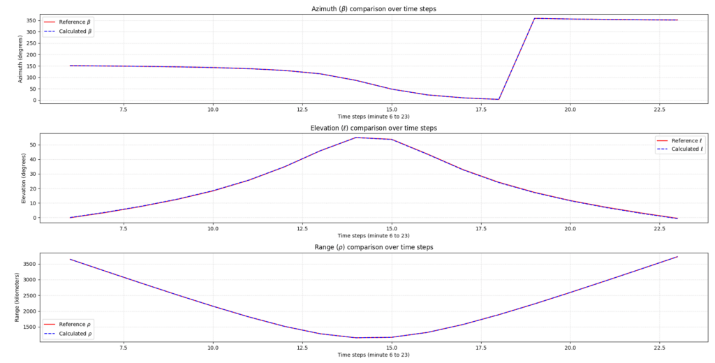
Execution time: 0.004263 s.At Fig. 1 shown the graphs representing Exercise 2.4.
Exercise 2.6 – Initial orbit determination
With ECEFtoLatLon algorithm from “Fundamentals” determining that the ground station is ISTARC ISRO, in Bengaluru, Karnataka, India. Then with SiteTrack determining state vectors at given moments, using JulianDate calculating actual , with LambertUniversalVariables solving Lambert problem, and with RV2COE determine orbit parameters.
Running Exercise_2_6.py...

Position vectors in given time
+----------+-----------+------------+-----------+-------------+-----------+
| Vector   |    i (km) |     j (km) |    k (km) |   mag. (km) |   α (deg) |
+==========+===========+============+===========+=============+===========+
| r1ref    | 11959.978 | -16289.478 | -5963.827 |       -     | -         |
+----------+-----------+------------+-----------+-------------+-----------+
| r1       | 11964.014 | -16286.739 | -5963.210 |       -     | -         |
+----------+-----------+------------+-----------+-------------+-----------+
| Δr1      |    -4.036 |     -2.739 |    -0.617 |       4.917 | 1.337e-02 |
+----------+-----------+------------+-----------+-------------+-----------+
| r2ref    | 39863.390 | -13730.547 | -4862.350 |       -     | -         |
+----------+-----------+------------+-----------+-------------+-----------+
| r2       | 39866.772 | -13721.910 | -4859.001 |       -     | -         |
+----------+-----------+------------+-----------+-------------+-----------+
| Δr2      |    -3.382 |     -8.637 |    -3.349 |       9.862 | 1.331e-02 |
+----------+-----------+------------+-----------+-------------+-----------+

Orbit parameters achieved with IOD
+--------------+---------------+---------------+--------------+
| Parameter    |    Ref. value |    Calculated |   Difference |
+==============+===============+===============+==============+
| a/SMA (km)   | 28196.78      | 28196.77      |    5.743e-03 |
+--------------+---------------+---------------+--------------+
| e/ECC        |     0.7679436 |     0.7679438 |    1.565e-07 |
+--------------+---------------+---------------+--------------+
| i/INC (deg)  |    20.315     |    20.31721   |    2.209e-03 |
+--------------+---------------+---------------+--------------+
| Ω/RAAN (deg) |   359.145     |   359.1421    |    2.885e-03 |
+--------------+---------------+---------------+--------------+
| ω/AOP (deg)  |   179.425     |   179.4409    |    1.590e-02 |
+--------------+---------------+---------------+--------------+
| M/MA (deg)   |    29.236     |    29.2362    |    2.000e-04 |
+--------------+---------------+---------------+--------------+
Execution time: 0.003390 s.Exercise 3.1 – Gravity field calculation
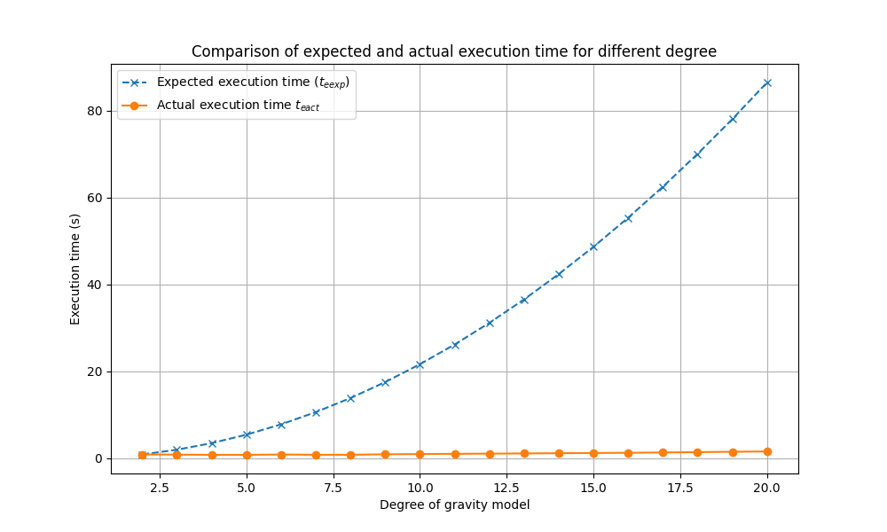
The goal was to calculate non-spherical acceleration at given point using Cunningham algorithm and compare it with reference (quadratic) complexity growth. I am not using Cunningham algorithm – instead I am using much more advanced algorithm based on data provided in “Fundamentals”. It is way more precise, and way faster (especially when it is multi-threading and made with C++ 😆)!
Here is the table with results:
Running Exercise_3_1.py...
Expected and actual execution times
+----------+-------------------+-----------------+
|   Degree |   Expected te (s) |   Actual te (s) |
+==========+===================+=================+
|        2 |             0.847 |           0.847 |
+----------+-------------------+-----------------+
|        3 |             1.905 |           0.801 |
+----------+-------------------+-----------------+
|        4 |             3.388 |           0.781 |
+----------+-------------------+-----------------+
|        5 |             5.293 |           0.847 |
+----------+-------------------+-----------------+
|        6 |             7.622 |           0.879 |
+----------+-------------------+-----------------+
|        7 |            10.374 |           0.772 |
+----------+-------------------+-----------------+
|        8 |            13.550 |           0.784 |
+----------+-------------------+-----------------+
|        9 |            17.149 |           0.898 |
+----------+-------------------+-----------------+
|       10 |            21.172 |           0.959 |
+----------+-------------------+-----------------+
|       11 |            25.618 |           1.002 |
+----------+-------------------+-----------------+
|       12 |            30.488 |           1.047 |
+----------+-------------------+-----------------+
|       13 |            35.781 |           1.091 |
+----------+-------------------+-----------------+
|       14 |            41.497 |           1.136 |
+----------+-------------------+-----------------+
|       15 |            47.637 |           1.192 |
+----------+-------------------+-----------------+
|       16 |            54.200 |           1.253 |
+----------+-------------------+-----------------+
|       17 |            61.187 |           1.316 |
+----------+-------------------+-----------------+
|       18 |            68.597 |           1.392 |
+----------+-------------------+-----------------+
|       19 |            76.431 |           1.473 |
+----------+-------------------+-----------------+
|       20 |            84.688 |           1.544 |
+----------+-------------------+-----------------+That’s the performance! As you can see, the time graph of my algorithm is almost flat. The graph at Fig. 2 shows this effect especially good:
Exercise 3.2 – Moon ephemerides
Utilizing series solution provided in “Fundamentals”, achieving:
Running Exercise_3_2.py...
Deviations of Moon position in comparison with analytics solution and ephemeris reference
+---------------------+----------------------+----------------------+
| Date/time UTC       |   Deviation C-A (km) |   Deviation C-E (km) |
+=====================+======================+======================+
| 2006/03/14 00:00:00 |             1521.407 |             1538.032 |
+---------------------+----------------------+----------------------+
| 2006/03/15 00:00:00 |             1814.177 |             1835.210 |
+---------------------+----------------------+----------------------+
| 2006/03/16 00:00:00 |             2003.893 |             2010.472 |
+---------------------+----------------------+----------------------+
| 2006/03/17 00:00:00 |             2051.150 |             2036.228 |
+---------------------+----------------------+----------------------+
| 2006/03/18 00:00:00 |             1941.834 |             1911.657 |
+---------------------+----------------------+----------------------+

Root Mean Square Error
+-----------------+-----------------+
|   RMSE C-A (km) |   RMSE C-E (km) |
+=================+=================+
|        1876.137 |        1874.897 |
+-----------------+-----------------+

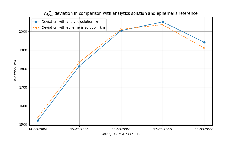
Execution time: 0.000364 s.Well, fast, but with deviation about 1 radius of the Moon itself… Graph at Fig. 3 shows the problem:
The algorithm definitely needs improvements. But for everyday purposes it’s enough – we’re not flying to the Moon so often…
Exercise 3.4 – Orbit perturbations
For force model for this task were used:
- J2-J6 (for GM order/degree 2/0) and EGM 2008 gravity models
- IAU76 FK5 ECI<–>ECEF coordinate conversion
- exponential atmosphere model
- n-body gravity model as described in “Fundamentals of Astrodynamics and Applications”,
- simple SRP model presented in the same textbook
Integration of motion processed in Python with RK4 (that’s why so slow).
I allowed myself to shorten the task and omitted part of the answers, but even existing answers provide very representative view:
Running Exercise_3_4.py...
Preparing initial data...
Non-perturbed (Kepler) propagation calculated in [ms]: 0.023

Expected calculated deviation from Kepler motion after 1 turn in LEO (depending on calculation parameters)
+-------------+------------+-------+--------+--------+-------+------------------+----------------------+
|   GM degree |   GM order | Sun   | Moon   | Drag   | SRP   |   Deviation (km) |   Execution time (s) |
+=============+============+=======+========+========+=======+==================+======================+
|           2 |          0 | False | False  | False  | False |           32.144 |                0.470 |
+-------------+------------+-------+--------+--------+-------+------------------+----------------------+
|           2 |          2 | False | False  | False  | False |           32.585 |                0.460 |
+-------------+------------+-------+--------+--------+-------+------------------+----------------------+
|           4 |          4 | False | False  | False  | False |           32.599 |                0.472 |
+-------------+------------+-------+--------+--------+-------+------------------+----------------------+
|          10 |         10 | False | False  | False  | False |           32.519 |                0.514 |
+-------------+------------+-------+--------+--------+-------+------------------+----------------------+
|          10 |         10 | True  | False  | False  | False |           32.518 |                0.526 |
+-------------+------------+-------+--------+--------+-------+------------------+----------------------+
|          10 |         10 | True  | True   | False  | False |           32.517 |                0.539 |
+-------------+------------+-------+--------+--------+-------+------------------+----------------------+
|          10 |         10 | True  | True   | True   | False |           32.517 |                0.556 |
+-------------+------------+-------+--------+--------+-------+------------------+----------------------+
|          10 |         10 | True  | True   | True   | True  |           32.518 |                0.555 |
+-------------+------------+-------+--------+--------+-------+------------------+----------------------+

Updating initial data...
Non-perturbed (Kepler) propagation calculated in [ms]: 0.034

Expected calculated deviation from Kepler motion after 1 turn in GEO (depending on calculation parameters)
+-------------+------------+-------+--------+--------+-------+------------------+----------------------+
|   GM degree |   GM order | Sun   | Moon   | Drag   | SRP   |   Deviation (km) |   Execution time (s) |
+=============+============+=======+========+========+=======+==================+======================+
|           2 |          0 | False | False  | False  | False |           19.726 |                0.654 |
+-------------+------------+-------+--------+--------+-------+------------------+----------------------+
|           2 |          2 | False | False  | False  | False |           20.379 |                0.663 |
+-------------+------------+-------+--------+--------+-------+------------------+----------------------+
|           4 |          4 | False | False  | False  | False |           20.380 |                0.651 |
+-------------+------------+-------+--------+--------+-------+------------------+----------------------+
|          10 |         10 | False | False  | False  | False |           20.379 |                0.727 |
+-------------+------------+-------+--------+--------+-------+------------------+----------------------+
|          10 |         10 | True  | False  | False  | False |           18.770 |                0.740 |
+-------------+------------+-------+--------+--------+-------+------------------+----------------------+
|          10 |         10 | True  | True   | False  | False |           11.694 |                0.779 |
+-------------+------------+-------+--------+--------+-------+------------------+----------------------+
|          10 |         10 | True  | True   | True   | False |           11.694 |                0.797 |
+-------------+------------+-------+--------+--------+-------+------------------+----------------------+
|          10 |         10 | True  | True   | True   | True  |           12.090 |                0.796 |
+-------------+------------+-------+--------+--------+-------+------------------+----------------------+Exercise 4.1 – 4th-order Runge–Kutta method
Perfect match.
Running Exercise_4_1.py...
Assess of accuracy of RK4 algorithm depending on number of steps
+---------+-----------+-----------+--------------+
|   Steps |    Ref. Δ |         Δ |   Difference |
+=========+===========+===========+==============+
|     200 | 1.953e-01 | 1.953e-01 |    4.826e-05 |
+---------+-----------+-----------+--------------+
|     400 | 6.663e-03 | 6.663e-03 |    2.674e-07 |
+---------+-----------+-----------+--------------+
|    1000 | 9.051e-05 | 9.051e-05 |    2.520e-10 |
+---------+-----------+-----------+--------------+
|    2000 | 4.012e-06 | 4.012e-06 |    4.595e-11 |
+---------+-----------+-----------+--------------+
|    3000 | 6.847e-07 | 6.847e-07 |    2.291e-11 |
+---------+-----------+-----------+--------------+
|    4000 | 1.996e-07 | 1.996e-07 |    4.207e-11 |
+---------+-----------+-----------+--------------+
|    6000 | 3.608e-08 | 3.608e-08 |    2.736e-12 |
+---------+-----------+-----------+--------------+
|    8000 | 1.089e-08 | 1.089e-08 |    3.233e-12 |
+---------+-----------+-----------+--------------+

Execution time: 0.243464 s.Exercise 4.2 – 4th-order Gauss–Jackson method
I did not implement exact Gauss-Jackson integration algorithm. Instead I implemented non-summed difference MultiStep Fixed Step Dual Integration Predictor-Corrector algorithm (MSFSDIPC), and also Adams-Bashforth-Moulton and other specialized integration algorithms.
All methods were set to 4-th order.
Here are the results:
Running Exercise_4_2.py...
Assess of accuracy of MSFSDIPC algorithm (Adams-Bashforth/Moulton & Stormer/Cowell) depending on number of steps
+---------+-----------+-----------+--------------+
|   Steps |    Ref. Δ |         Δ |   Difference |
+=========+===========+===========+==============+
|     100 | 2.456e-03 | 6.876e-03 |    4.420e-03 |
+---------+-----------+-----------+--------------+
|     300 | 3.363e-06 | 8.360e-05 |    8.024e-05 |
+---------+-----------+-----------+--------------+
|     600 | 7.705e-08 | 5.216e-06 |    5.139e-06 |
+---------+-----------+-----------+--------------+
|    1000 | 4.539e-09 | 6.758e-07 |    6.712e-07 |
+---------+-----------+-----------+--------------+
|    1500 | 5.174e-10 | 1.336e-07 |    1.331e-07 |
+---------+-----------+-----------+--------------+
|    2000 | 1.166e-10 | 4.224e-08 |    4.212e-08 |
+---------+-----------+-----------+--------------+
|    3000 | 1.499e-11 | 8.345e-09 |    8.330e-09 |
+---------+-----------+-----------+--------------+
|    4000 | 3.577e-12 | 2.649e-09 |    2.646e-09 |
+---------+-----------+-----------+--------------+

Execution time: 1.232893 s.

Assess of accuracy of MSFSSIPC algorithm (Adams-Bashforth-Moulton) depending on number of steps
+---------+-----------+-----------+--------------+
|   Steps |    Ref. Δ |         Δ |   Difference |
+=========+===========+===========+==============+
|     100 | 2.456e-03 | 9.490e-03 |    7.034e-03 |
+---------+-----------+-----------+--------------+
|     300 | 3.363e-06 | 2.953e-04 |    2.920e-04 |
+---------+-----------+-----------+--------------+
|     600 | 7.705e-08 | 2.099e-05 |    2.092e-05 |
+---------+-----------+-----------+--------------+
|    1000 | 4.539e-09 | 2.937e-06 |    2.932e-06 |
+---------+-----------+-----------+--------------+
|    1500 | 5.174e-10 | 5.605e-07 |    5.600e-07 |
+---------+-----------+-----------+--------------+
|    2000 | 1.166e-10 | 8.154e-08 |    8.142e-08 |
+---------+-----------+-----------+--------------+
|    3000 | 1.499e-11 | 2.315e-08 |    2.313e-08 |
+---------+-----------+-----------+--------------+
|    4000 | 3.577e-12 | 8.452e-09 |    8.448e-09 |
+---------+-----------+-----------+--------------+

Execution time: 0.637043 s.

Assess of accuracy of FSSIP algorithm (Adams-Bashforth) depending on number of steps
+---------+-----------+-----------+--------------+
|   Steps |    Ref. Δ |         Δ |   Difference |
+=========+===========+===========+==============+
|     100 | 2.456e-03 | 1.926e-01 |    1.901e-01 |
+---------+-----------+-----------+--------------+
|     300 | 3.363e-06 | 2.826e-03 |    2.822e-03 |
+---------+-----------+-----------+--------------+
|     600 | 7.705e-08 | 2.453e-04 |    2.452e-04 |
+---------+-----------+-----------+--------------+
|    1000 | 4.539e-09 | 3.519e-05 |    3.518e-05 |
+---------+-----------+-----------+--------------+
|    1500 | 5.174e-10 | 7.277e-06 |    7.277e-06 |
+---------+-----------+-----------+--------------+
|    2000 | 1.166e-10 | 2.354e-06 |    2.353e-06 |
+---------+-----------+-----------+--------------+
|    3000 | 1.499e-11 | 4.749e-07 |    4.749e-07 |
+---------+-----------+-----------+--------------+
|    4000 | 3.577e-12 | 1.518e-07 |    1.518e-07 |
+---------+-----------+-----------+--------------+

Execution time: 0.273475 s.As you can see, accuracy is comparable with RK4.
I did not understand yet how Mr. Montenbruck achieved . Maybe the roots of the problem caused by usage non-summed and difference (not ordinated) version of multistep integrators. This problem requires further studies.
Exercise 5.2 – Velocity in the Earth-fixed frame
Quite simple. Using Vallado’s IAU76FK5 with proper EOP parameters, and RV2COE, achieving:
Running Exercise_5_2.py...
Results of position vector conversion (WGS->ICRS)
+------------+------------+-----------+-----------+-----------+
| Vector     |     I (km) |    J (km) |    K (km) |    Δ (km) |
+============+============+===========+===========+===========+
| rICRS ref. | -23830.593 | -9747.074 | -6779.829 | -         |
+------------+------------+-----------+-----------+-----------+
| rICRS      | -23830.593 | -9747.074 | -6779.831 | 2.162e-03 |
+------------+------------+-----------+-----------+-----------+

Results of velocity vector conversion (WGS->ICRS)
+------------+------------+------------+------------+------------+
| Vector     |   I (km/s) |   J (km/s) |   K (km/s) |   Δ (km/s) |
+============+============+============+============+============+
| vICRS ref. |      1.562 |     -1.754 |     -3.069 |  -         |
+------------+------------+------------+------------+------------+
| vICRS      |      1.562 |     -1.754 |     -3.069 |  9.457e-07 |
+------------+------------+------------+------------+------------+

Orbit parameters calculated from ICRS state vectors
+--------------+---------------+-----------------+--------------+
| Parameter    |    Ref. value |      Calculated |   Difference |
+==============+===============+=================+==============+
| a/SMA (km)   | 26561.01      | 26561.01        |    1.401e-04 |
+--------------+---------------+-----------------+--------------+
| e/ECC        |     0.0070606 |     0.007060631 |    3.064e-08 |
+--------------+---------------+-----------------+--------------+
| i/INC (deg)  |    56.338     |    56.33828     |    2.835e-04 |
+--------------+---------------+-----------------+--------------+
| Ω/RAAN (deg) |    12.146     |    12.14554     |    4.561e-04 |
+--------------+---------------+-----------------+--------------+
| ω/AOP (deg)  |    87.617     |    87.61883     |    1.828e-03 |
+--------------+---------------+-----------------+--------------+
| M/MA (deg)   |   109.435     |   109.4355      |    4.648e-04 |
+--------------+---------------+-----------------+--------------+

Execution time: 0.002857 s.Exercise 5.3 – Geodetic coordinates
Again, quite simple.
Running Exercise_5_3.py...

Geodetic coordinates calculated from WGS position vector
+-------------+--------------+--------------+--------------+
| Parameter   |   Ref. value |   Calculated |   Difference |
+=============+==============+==============+==============+
| φgd (deg)   |    -7.26655  |    -7.26655  |    1.794e-08 |
+-------------+--------------+--------------+--------------+
| λ (deg)     |    72.363121 |    72.363121 |    2.485e-09 |
+-------------+--------------+--------------+--------------+
| h ellip m   |   -63.667    |   -63.666726 |    2.741e-04 |
+-------------+--------------+--------------+--------------+

Execution time: 0.000087 s.Conclusions
Tests on exercises from the textbook of Mr. Montenbruck showed that my astrodynamics toolset software library is acceptable for practical purposes (despite it still has number of problems).
Moon position calculation algorithm requires deep refactoring, using other solution than provided in “Fundamentals of Astrodynamics and Applications”.
Questions of usage of multi-step integration algorithms requires further studies.