Multi-step integration – practical test

Preface

Earlier, I undertook a validation testing of algorithms form my astrodynamics software tools library. Briefly, it showed that my algorithms are valid and suitable for practical purposes. But despite this they have number of questionable properties. One of such features was linked with multi-step integration algorithms (also known as family of Störmer-Cowell & Gauss-Jackson integration methods).

Bug or feature?

In a nutshell, the problem was in precision of my implementation of multi-step integration algorithm.

In textbook “Satellite Orbits. Models, Methods and Applications” © 2000 by Oliver Montenbruck & Eberhard Gill, especially in Exercise 4.2, the task was to complete the integration of motion ODE using 4-th order Gauss-Jackson integration method, described earlier in this book.

I did not implement the method described by Mr. Montenbruck, but rely on method based on one explained in “Fundamentals of Astrodynamics and Applications”, Fourth Edition, by David A. Vallado. I named this implementation MSFSDIPC – Multi-Step Fixed Step Dual Integration Predictor-Corrector.

Solution with this method provided questionable result. Here is the output from solution of Exercise 4.2:

Running Exercise_4_2.py...
Assess of accuracy of MSFSDIPC algorithm (Adams-Bashforth/Moulton & Stormer/Cowell) depending on number of steps
+---------+-----------+-----------+--------------+
|   Steps |    Ref. Δ |         Δ |   Difference |
+=========+===========+===========+==============+
|     100 | 2.456e-03 | 6.876e-03 |    4.420e-03 |
+---------+-----------+-----------+--------------+
|     300 | 3.363e-06 | 8.360e-05 |    8.024e-05 |
+---------+-----------+-----------+--------------+
|     600 | 7.705e-08 | 5.216e-06 |    5.139e-06 |
+---------+-----------+-----------+--------------+
|    1000 | 4.539e-09 | 6.758e-07 |    6.712e-07 |
+---------+-----------+-----------+--------------+
|    1500 | 5.174e-10 | 1.336e-07 |    1.331e-07 |
+---------+-----------+-----------+--------------+
|    2000 | 1.166e-10 | 4.224e-08 |    4.212e-08 |
+---------+-----------+-----------+--------------+
|    3000 | 1.499e-11 | 8.345e-09 |    8.330e-09 |
+---------+-----------+-----------+--------------+
|    4000 | 3.577e-12 | 2.649e-09 |    2.646e-09 |
+---------+-----------+-----------+--------------+

Execution time: 1.232893 s.

Running Exercise_4_2.py...
Assess of accuracy of MSFSDIPC algorithm (Adams-Bashforth/Moulton & Stormer/Cowell) depending on number of steps
+---------+-----------+-----------+--------------+
|   Steps |    Ref. Δ |         Δ |   Difference |
+=========+===========+===========+==============+
|     100 | 2.456e-03 | 6.876e-03 |    4.420e-03 |
+---------+-----------+-----------+--------------+
|     300 | 3.363e-06 | 8.360e-05 |    8.024e-05 |
+---------+-----------+-----------+--------------+
|     600 | 7.705e-08 | 5.216e-06 |    5.139e-06 |
+---------+-----------+-----------+--------------+
|    1000 | 4.539e-09 | 6.758e-07 |    6.712e-07 |
+---------+-----------+-----------+--------------+
|    1500 | 5.174e-10 | 1.336e-07 |    1.331e-07 |
+---------+-----------+-----------+--------------+
|    2000 | 1.166e-10 | 4.224e-08 |    4.212e-08 |
+---------+-----------+-----------+--------------+
|    3000 | 1.499e-11 | 8.345e-09 |    8.330e-09 |
+---------+-----------+-----------+--------------+
|    4000 | 3.577e-12 | 2.649e-09 |    2.646e-09 |
+---------+-----------+-----------+--------------+

Execution time: 1.232893 s.

Before we will continue, compare it with output of solution of the Exercise 4.1, where we must solve same problem using generic 4-th order Runge-Kutta integrator:

Running Exercise_4_1.py...
Assess of accuracy of RK4 algorithm depending on number of steps
+---------+-----------+-----------+--------------+
|   Steps |    Ref. Δ |         Δ |   Difference |
+=========+===========+===========+==============+
|     200 | 1.953e-01 | 1.953e-01 |    4.826e-05 |
+---------+-----------+-----------+--------------+
|     400 | 6.663e-03 | 6.663e-03 |    2.674e-07 |
+---------+-----------+-----------+--------------+
|    1000 | 9.051e-05 | 9.051e-05 |    2.520e-10 |
+---------+-----------+-----------+--------------+
|    2000 | 4.012e-06 | 4.012e-06 |    4.595e-11 |
+---------+-----------+-----------+--------------+
|    3000 | 6.847e-07 | 6.847e-07 |    2.291e-11 |
+---------+-----------+-----------+--------------+
|    4000 | 1.996e-07 | 1.996e-07 |    4.207e-11 |
+---------+-----------+-----------+--------------+
|    6000 | 3.608e-08 | 3.608e-08 |    2.736e-12 |
+---------+-----------+-----------+--------------+
|    8000 | 1.089e-08 | 1.089e-08 |    3.233e-12 |
+---------+-----------+-----------+--------------+

Execution time: 0.246442 s.

Running Exercise_4_1.py...
Assess of accuracy of RK4 algorithm depending on number of steps
+---------+-----------+-----------+--------------+
|   Steps |    Ref. Δ |         Δ |   Difference |
+=========+===========+===========+==============+
|     200 | 1.953e-01 | 1.953e-01 |    4.826e-05 |
+---------+-----------+-----------+--------------+
|     400 | 6.663e-03 | 6.663e-03 |    2.674e-07 |
+---------+-----------+-----------+--------------+
|    1000 | 9.051e-05 | 9.051e-05 |    2.520e-10 |
+---------+-----------+-----------+--------------+
|    2000 | 4.012e-06 | 4.012e-06 |    4.595e-11 |
+---------+-----------+-----------+--------------+
|    3000 | 6.847e-07 | 6.847e-07 |    2.291e-11 |
+---------+-----------+-----------+--------------+
|    4000 | 1.996e-07 | 1.996e-07 |    4.207e-11 |
+---------+-----------+-----------+--------------+
|    6000 | 3.608e-08 | 3.608e-08 |    2.736e-12 |
+---------+-----------+-----------+--------------+
|    8000 | 1.089e-08 | 1.089e-08 |    3.233e-12 |
+---------+-----------+-----------+--------------+

Execution time: 0.246442 s.

As you can see, MSFSDIPC execution time is almost exactly $5$ times longer one of RK4, and overall accuracy (especially at higher steps count – i.e., on smaller steps) is not much higher.

On the other hand, actual accuracy of MSFSDIPC on smaller steps count are much higher – for step count 100 it’s $\approx{28.4}$ times higher than for RK4!

Despite this, mentioned phenomena required deeper studies.

Practical test

The statement “practice is the criterion of truth” was formulated in political essays of Mao Tse-tung. In marxist theory, practice always been placed higher than theoretical knowledge. Marx, Lenin and Mao Tse-tung number of times mentioned about this in their works. Of course, in their case it was populism blabbing pursuing political reasons. But the statement itself is rational – at least in some cases.

So, by my opinion, practical test (i.e., experiment) can give information able to proof the correctness of MSFSDIPC algorithm.

Experiment set up

Goal and initial hypothesis

The goal of an experiment were to check on real data precision of my MSFSDIPC integrator. The hypothesis of the experiment was in that my integration algorithm, implemented on the basis of the instructions from “Fundamentals” will have advantages over standard Runge-Kutta method. But exact traits of these advantages were not clear for me at that moment.

Subject

At the moment I had a good EGM 2008 gravity model implementation, but no precise atmospheric model. Additionally, in “Fundamentals of Astrodynamics and Applications” Mr. Vallado mentioned that multi-step integration algorithms are bad for accurate propagation at highly elliptic orbits.

Thus, the “subject” for experiment was chosen – I needed a well-known, carefully tracked MEO satellite, which fly far enough from atmospheric disturbance on the circular orbit. One of GPS satellites looked as a perfect choice to assess accuracy of my algorithm.

So I chose NAVSTAR 86. Here’s its TLE of for 11.09.2026 – 14.09.2026:

#Position for NAVSTAR 86 (NORAD ID 68791), from space-track.org
# --- First state ---
'''
===== TLE =====
1 68791U 26087A   26254.39889477 -.00000012  00000-0  00000-0 0  9992
2 68791  54.9553 204.3810 0021324 102.9910  67.7109  2.00577427  2563
'''

'''
===== RV =====
Error: 0
JD: 2461294.89889477
UTC: 2026 9 11 9 34 24.508128
R: [24857.66857639  8648.7396268   3392.97227445]
V: [-0.34757577  2.2551253  -3.13488258]
'''

# --- Second state
'''
===== TLE =====
1 68791U 26087A   26257.40036010  .00000015  00000-0  00000-0 0  9996
2 68791  54.9549 204.2625 0021537 102.5730  75.4972  2.00577731  2622
'''

'''
===== RV =====
Error: 0
JD: 2461297.9003601
UTC: 2026 9 14 9 36 31.11264
R: [24369.32488925 10507.02369762   613.34284096]
V: [-0.80549864  2.07613598 -3.17265984]
'''

#Position for NAVSTAR 86 (NORAD ID 68791), from space-track.org
# --- First state ---
'''
===== TLE =====
1 68791U 26087A   26254.39889477 -.00000012  00000-0  00000-0 0  9992
2 68791  54.9553 204.3810 0021324 102.9910  67.7109  2.00577427  2563
'''

'''
===== RV =====
Error: 0
JD: 2461294.89889477
UTC: 2026 9 11 9 34 24.508128
R: [24857.66857639  8648.7396268   3392.97227445]
V: [-0.34757577  2.2551253  -3.13488258]
'''

# --- Second state
'''
===== TLE =====
1 68791U 26087A   26257.40036010  .00000015  00000-0  00000-0 0  9996
2 68791  54.9549 204.2625 0021537 102.5730  75.4972  2.00577731  2622
'''

'''
===== RV =====
Error: 0
JD: 2461297.9003601
UTC: 2026 9 14 9 36 31.11264
R: [24369.32488925 10507.02369762   613.34284096]
V: [-0.80549864  2.07613598 -3.17265984]
'''

UTC dates and state vectors for first and second states of the satellite were calculated from TLE using sgp4 2.25 Python package.

Algorithms

In the experiment I used two integration methods:

5/4-th order Runge-Kutta-Nyström (implemented following description from Wikipedia)
variable-order MSFSDIPC (implemented following description from “Fundamentals”)

Method

The method of an experiment was to compute propagation of the orbit of NAVSTAR 86, from first state to second state, using time steps 360, 600, 900, 1800 and 3600 sec.

For each of this time step settings, an experimental program will run:

RKN5/4 (using its default order 4)
MSFSDIPC with order 4, 8, and 12.

As a results the app will record:

$\Delta{r}$ (km) – distance between satellite position measured at second state and position calculated by propagation algorithms
$\Delta{v}$ (km/s) – difference between measured and calculated satellite velocity at second state.
$t_{exec}$ (s) – execution time required for calculation.

Gathered data will be analyzed for understanding advantages and flaws of both algorithms.

Force model

Force model for an experiment used:

EGM 2008 gravity model with order/degree 6×6
IAU76FK5 ECEF<–>ECI coordinate conversion algorithm
exponential atmosphere model
simple 3-body model of the gravity of Sun
simple 3-body model of the gravity of Moon
simple SRP model

All used models were based on description provided in “Fundamentals”.

Results of an experiment

Results of an experiment provided in a table below:

Comparison of precision and performance of RKN5 & MSFSDIPC integration algorithms
+-------------+---------+---------+-----------+-------------+---------------+
| Algorithm   |   h (s) | Order   |   Δr (km) |   Δv (km/s) |   t exec. (s) |
+=============+=========+=========+===========+=============+===============+
| RKN5        |     360 | 5/4     |     5.517 |       0.001 |      3.717507 |
+-------------+---------+---------+-----------+-------------+---------------+
| MSFSDIPC    |     360 | 4       |     5.425 |       0.001 |      2.945726 |
+-------------+---------+---------+-----------+-------------+---------------+
| MSFSDIPC    |     360 | 8       |     5.492 |       0.001 |      1.765162 |
+-------------+---------+---------+-----------+-------------+---------------+
| MSFSDIPC    |     360 | 12      |     5.492 |       0.001 |      2.879853 |
+-------------+---------+---------+-----------+-------------+---------------+
| RKN5        |     600 | 5/4     |     5.768 |       0.001 |      2.266504 |
+-------------+---------+---------+-----------+-------------+---------------+
| MSFSDIPC    |     600 | 4       |     4.930 |       0.001 |      2.435654 |
+-------------+---------+---------+-----------+-------------+---------------+
| MSFSDIPC    |     600 | 8       |     5.447 |       0.001 |      1.503643 |
+-------------+---------+---------+-----------+-------------+---------------+
| MSFSDIPC    |     600 | 12      |     5.447 |       0.001 |      1.889308 |
+-------------+---------+---------+-----------+-------------+---------------+
| RKN5        |     900 | 5/4     |     7.837 |       0.001 |      1.506800 |
+-------------+---------+---------+-----------+-------------+---------------+
| MSFSDIPC    |     900 | 4       |     2.800 |       0.000 |      1.609958 |
+-------------+---------+---------+-----------+-------------+---------------+
| MSFSDIPC    |     900 | 8       |     5.427 |       0.001 |      1.462573 |
+-------------+---------+---------+-----------+-------------+---------------+
| MSFSDIPC    |     900 | 12      |     5.425 |       0.001 |      1.377960 |
+-------------+---------+---------+-----------+-------------+---------------+
| RKN5        |    1800 | 5/4     |    79.253 |       0.011 |      0.761792 |
+-------------+---------+---------+-----------+-------------+---------------+
| MSFSDIPC    |    1800 | 4       |    37.390 |       0.006 |      1.235582 |
+-------------+---------+---------+-----------+-------------+---------------+
| MSFSDIPC    |    1800 | 8       |     6.918 |       0.001 |      1.184883 |
+-------------+---------+---------+-----------+-------------+---------------+
| MSFSDIPC    |    1800 | 12      |     5.456 |       0.001 |      1.356234 |
+-------------+---------+---------+-----------+-------------+---------------+
| RKN5        |    3600 | 5/4     |  1923.175 |       0.280 |      0.402577 |
+-------------+---------+---------+-----------+-------------+---------------+
| MSFSDIPC    |    3600 | 4       |   710.439 |       0.105 |      0.940690 |
+-------------+---------+---------+-----------+-------------+---------------+
| MSFSDIPC    |    3600 | 8       |   743.089 |       0.109 |      1.013956 |
+-------------+---------+---------+-----------+-------------+---------------+
| MSFSDIPC    |    3600 | 12      |    63.244 |       0.008 |      1.289376 |
+-------------+---------+---------+-----------+-------------+---------------+

Comparison of precision and performance of RKN5 & MSFSDIPC integration algorithms
+-------------+---------+---------+-----------+-------------+---------------+
| Algorithm   |   h (s) | Order   |   Δr (km) |   Δv (km/s) |   t exec. (s) |
+=============+=========+=========+===========+=============+===============+
| RKN5        |     360 | 5/4     |     5.517 |       0.001 |      3.717507 |
+-------------+---------+---------+-----------+-------------+---------------+
| MSFSDIPC    |     360 | 4       |     5.425 |       0.001 |      2.945726 |
+-------------+---------+---------+-----------+-------------+---------------+
| MSFSDIPC    |     360 | 8       |     5.492 |       0.001 |      1.765162 |
+-------------+---------+---------+-----------+-------------+---------------+
| MSFSDIPC    |     360 | 12      |     5.492 |       0.001 |      2.879853 |
+-------------+---------+---------+-----------+-------------+---------------+
| RKN5        |     600 | 5/4     |     5.768 |       0.001 |      2.266504 |
+-------------+---------+---------+-----------+-------------+---------------+
| MSFSDIPC    |     600 | 4       |     4.930 |       0.001 |      2.435654 |
+-------------+---------+---------+-----------+-------------+---------------+
| MSFSDIPC    |     600 | 8       |     5.447 |       0.001 |      1.503643 |
+-------------+---------+---------+-----------+-------------+---------------+
| MSFSDIPC    |     600 | 12      |     5.447 |       0.001 |      1.889308 |
+-------------+---------+---------+-----------+-------------+---------------+
| RKN5        |     900 | 5/4     |     7.837 |       0.001 |      1.506800 |
+-------------+---------+---------+-----------+-------------+---------------+
| MSFSDIPC    |     900 | 4       |     2.800 |       0.000 |      1.609958 |
+-------------+---------+---------+-----------+-------------+---------------+
| MSFSDIPC    |     900 | 8       |     5.427 |       0.001 |      1.462573 |
+-------------+---------+---------+-----------+-------------+---------------+
| MSFSDIPC    |     900 | 12      |     5.425 |       0.001 |      1.377960 |
+-------------+---------+---------+-----------+-------------+---------------+
| RKN5        |    1800 | 5/4     |    79.253 |       0.011 |      0.761792 |
+-------------+---------+---------+-----------+-------------+---------------+
| MSFSDIPC    |    1800 | 4       |    37.390 |       0.006 |      1.235582 |
+-------------+---------+---------+-----------+-------------+---------------+
| MSFSDIPC    |    1800 | 8       |     6.918 |       0.001 |      1.184883 |
+-------------+---------+---------+-----------+-------------+---------------+
| MSFSDIPC    |    1800 | 12      |     5.456 |       0.001 |      1.356234 |
+-------------+---------+---------+-----------+-------------+---------------+
| RKN5        |    3600 | 5/4     |  1923.175 |       0.280 |      0.402577 |
+-------------+---------+---------+-----------+-------------+---------------+
| MSFSDIPC    |    3600 | 4       |   710.439 |       0.105 |      0.940690 |
+-------------+---------+---------+-----------+-------------+---------------+
| MSFSDIPC    |    3600 | 8       |   743.089 |       0.109 |      1.013956 |
+-------------+---------+---------+-----------+-------------+---------------+
| MSFSDIPC    |    3600 | 12      |    63.244 |       0.008 |      1.289376 |
+-------------+---------+---------+-----------+-------------+---------------+

Brief analysis of the table show that MSFSDIPC has expected advantage over RKN5 algorithm. It is visible even better, if we will present the results in a graphical form. Take a look on Fig. 1:

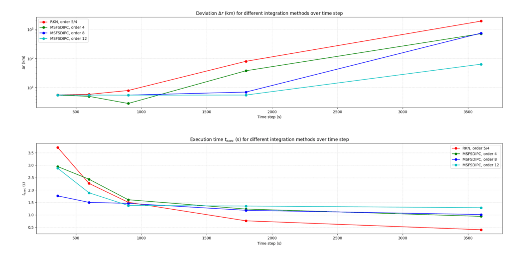
Note, that deviation (upper) plot presented in logarithmic scale!

Here is clearly visible that:

At smaller time steps MSFSDIPC is from $1.26$ to $2.70$ times faster than RKN5
At longer time steps MSFSDIPC does not loose precision even in cases where RKN “explodes”.

Last statement is clearly visible at time steps 1800 and 3600 seconds. Despite RKN5 is from $2.34$ to $3.20$ times faster here, MSFSDIPC is $14.5$ to $352.5$ times more accurate than RKN5.

Absolute error for position (if we omit terminal values at very high time steps) stays within $\approx 5.5$ kilometers. Getting in count relatively low TLE accuracy (where deviations for MEO can count 1.0 – 3.0 km), and propagation duration (about 3 days), we may say that accuracy achieved by MSFSDIPC is acceptable for rough astrogation even in that cases when RKN5 totally “lost in space”.

Conclusions

Described experiment showed that multi-step integration algorithm based on Adams-Bashforth-Moulton-, Störmer-Cowell and Gauss-Jackson methods described in “Fundamentals of Astrodynamics and Applications” is valid and applicable for practical astrodynamics applications, providing accuracy enough for practical operations.

To be honest, this is an expected result. In “Fundamentals” Mr. Vallado number of times mentioned that family of fixed-step-size multi-step integration methods are most optimal and most common for calculating of a propagation in stable circular orbits.

Obtained numeric values are also expected. At the bottom of p. 527 of the “Fundamentals” we have clear mention:

Herrick comments (1972) that for near-circular, near-Earth orbits, Gauss-Jackson is about one order of magnitude more efficient than a fourth-order Runge-Kutta

This is almost exactly the values I got.

Footnotes

Work on this experiment showed to me interesting traits of multi-step integration algorithms. They linked with variable time step problems and with generation of backpoints for MSFSDIPC algorithm. In my further notes I will describe this in more details.

ultradyne.space

Jacchia 71 atmosphere model

EGM 2008 2190 x 2159