Motivation

After implementation of EGM 2008, next logical step was to understand and implement algorithms simulating upper atmosphere of the Earth.

I understood that it will be hard, but remembering JFK’s “we’re doing this not because it’s easy…” (and following recommendations from my main textbook “Fundamentals of Astrodynamics and Applications”, Fourth Edition, by David Vallado) I decided to create my own C++-based implementation of an atmosphere model.

Options

Right after the start I faced a need to decide what exactly the model I should make? The thing is that there is wide variety of atmosphere models. Just using my memory, I can name:

• Jacchia 64
• Jacchia 71
• Jacchia 77
• Jacchia-Roberts
• Jacchia-Lineberry
• Jacchia-Bowmann 2008
• Jacchia-Gill
• MSISE-90
• NLRMSIS(E)-00
• COESA-76
• GOST 25645.115-84
• GOST 25645.166-2004
• etc.

Each of them describe upper Earth atmosphere with different degree of accuracy, many of them used in different astrodynamics software or simulations. Despite this, as far as I understand, none of them present “absolute” accuracy (because of dynamic nature of Earth atmosphere)

The choice was hard. Textbooks recommendations were controversial. Examples were limited and vague.

Decision

The help came from the textbook “Satellite Orbits. Models, Methods and Applications” © 2000 by Oliver Montenbruck & Eberhard Gill. There in Table 3.12 provided very useful comparison of accuracy and performance of different atmosphere models.

Following it and recommendation in Vallado’s “Fundamentals”, I chose for myself 4 main options to implement:

• Jacchia 71
• Jacchia-Roberts
• Jacchia-Gill
• GOST 25645.115-84

Here, Jacchia-Roberts looked too complex and thus useless in modern computation environment. Jacchia-Gill was good, but it was a simplified analytical version of original Jacchia model. And soviet GOST was very good, but it provided more narrow altitude boundaries than Jacchia.

So, this way I chose to implement original Jacchia 1971 atmospheric model.

Difficulties on coding

Implementation of Jacchia ’71 required lot of efforts. The model itself is simple and clear – when you understand it. The logic of the model is also not something special – by sense we baldly integrating composition of an atmosphere, calculating its density from temperature and specific amount of constituents.

But as always, “devil in details”, and details in original paper of Jacchia is described shortly and vague – or, better to say, just omitted.

Working code examples are rare, incomplete, and typically written in Fortran by “ancient titans in prehistoric times”.

And AIs, which everyone pray today so much, can not help here – because they just don’t understand what I am asking them about.

So I applied the method I already used many times – cross-testing between textbooks, Jacchia publications of 1964, 1971 and 1977, and modern research of mesopause and thermosphere, collected for me by AI. From this studies the idea of Jacchia model started to reveal in my mind.

Optimization

I tried to implement Jacchia ’71 model in different ways, using primitive and advanced integration techniques, but in the end I chose the simplest direct integration method. It provided good accuracy and relatively low computation overhead.

After deep optimization, including memory access optimization and implementation of multi-threading, I achieved very high performance of the system:

Release build performance:

Test mode	Pass number	Time (ms)
Static	13	5
Dynamic (static + all temperature corrections)	2	0.8

Results

In about a 2 weeks of tight work a full Jacchia ’71 atmospheric model was implemented. Implementation strictly followed description from “REVISED STATIC MODELS OF THE THERMOSPHERE AND EXOSPHERE WITH EMPIRICAL TEMPERATURE PROFILES” by L. G. Jacchia. ((c) Smithsonian Astrophysical Observatory * Provided by the NASA Astrophysics Data System) (1).

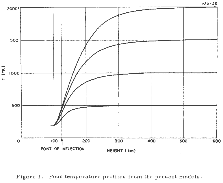
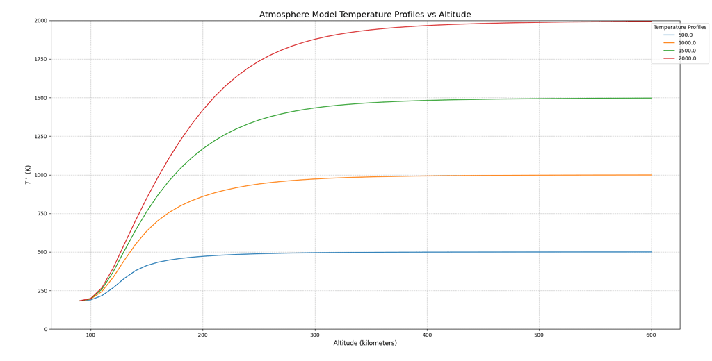
Model includes temperature profile model, strictly follows data from (1).

On Fig. #1 and #2 you can compare original profiles plot provided by Jacchia and a plot created on results of my implementation of the model:

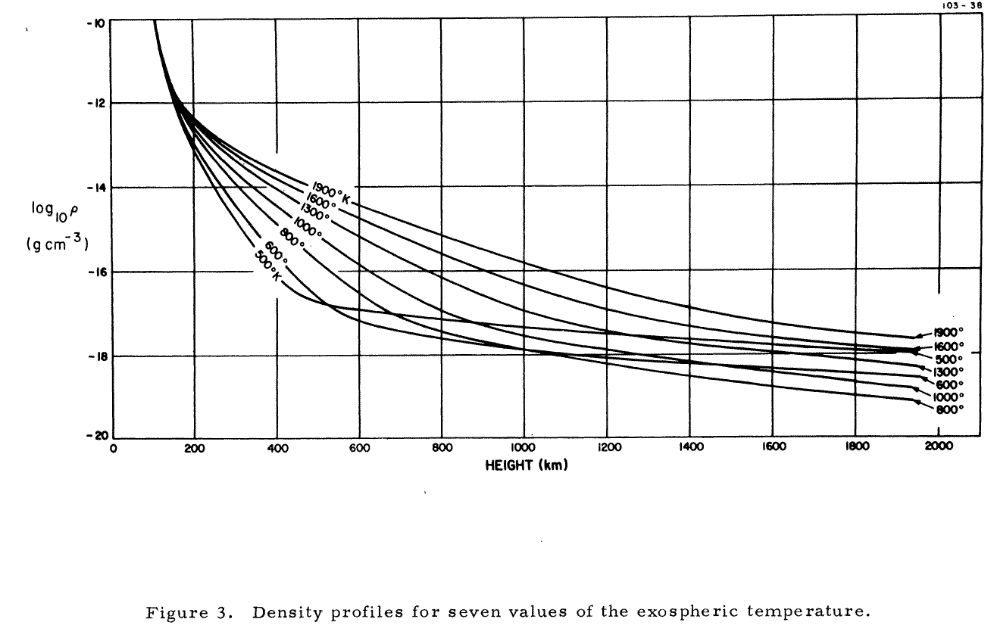
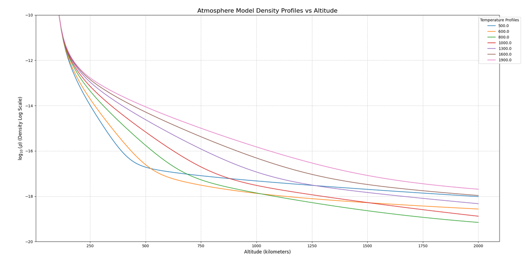
Further, model includes static composition model, also strictly follows data from (1).

On Fig. #3 and #4 you can compare original density profiles plot provided by Jacchia and a plot created on results of my implementation:

Using data created by temperature model and composition model, my algorithm calculates density of atmosphere on given altitude, applying all corrections, mentioned in (1), including:

• Temperature corrections for
  • Solar activity
  • Diurnal variation
  • Geomagnetic activity
• Density corrections for
  • Geomagnetic activity
  • Semiannual variation
  • Seasonal-latitudal variation
  • Helium numeric density

Exact match with Numeric Example, provided in (1) is not possible, because there Jacchia used rounded tabulated values and thus result of precise calculation will be different

Additionally algorithm provides precision control by ability of changing integration step size.

Integration step/accuracy:

Step (km)	$\Delta\log10(\rho)$ (g/cm^3)	Max altitude (km)
0.25	1e-3	2500
0.05	1e-4	~350
0.025	1e-4	~900
0.01	1e-4	~2250

Further steps

1. Improve accuracy of the model at higher altitudes
2. Compare accuracy and performance with other implementations of Jacchia family models and other atmosphere models
3. Test my implementation of Jacchia ’71 model on real data
4. Implement GOST 25645.115-84 atmosphere model as backup solution.